
Study Notes
Overview
Cubic graphs represent functions where the highest power of the variable (usually x) is 3, such as y = x³ or y = 2x³ - 3x + 1. For your Edexcel GCSE Mathematics exam, a solid understanding of cubic graphs is essential as it tests a combination of skills: accurate calculation, precise plotting, and graphical interpretation. These questions are a great opportunity to demonstrate your mathematical dexterity and secure a significant number of marks. On the Foundation tier, you will typically be asked to complete a table of values and plot a given cubic function. On the Higher tier, you may also be expected to sketch cubic graphs by identifying their roots and key features without a table. This topic has strong synoptic links to solving equations and understanding transformations of graphs, making it a cornerstone of algebra.
Key Concepts
Concept 1: The Shape of a Cubic Curve
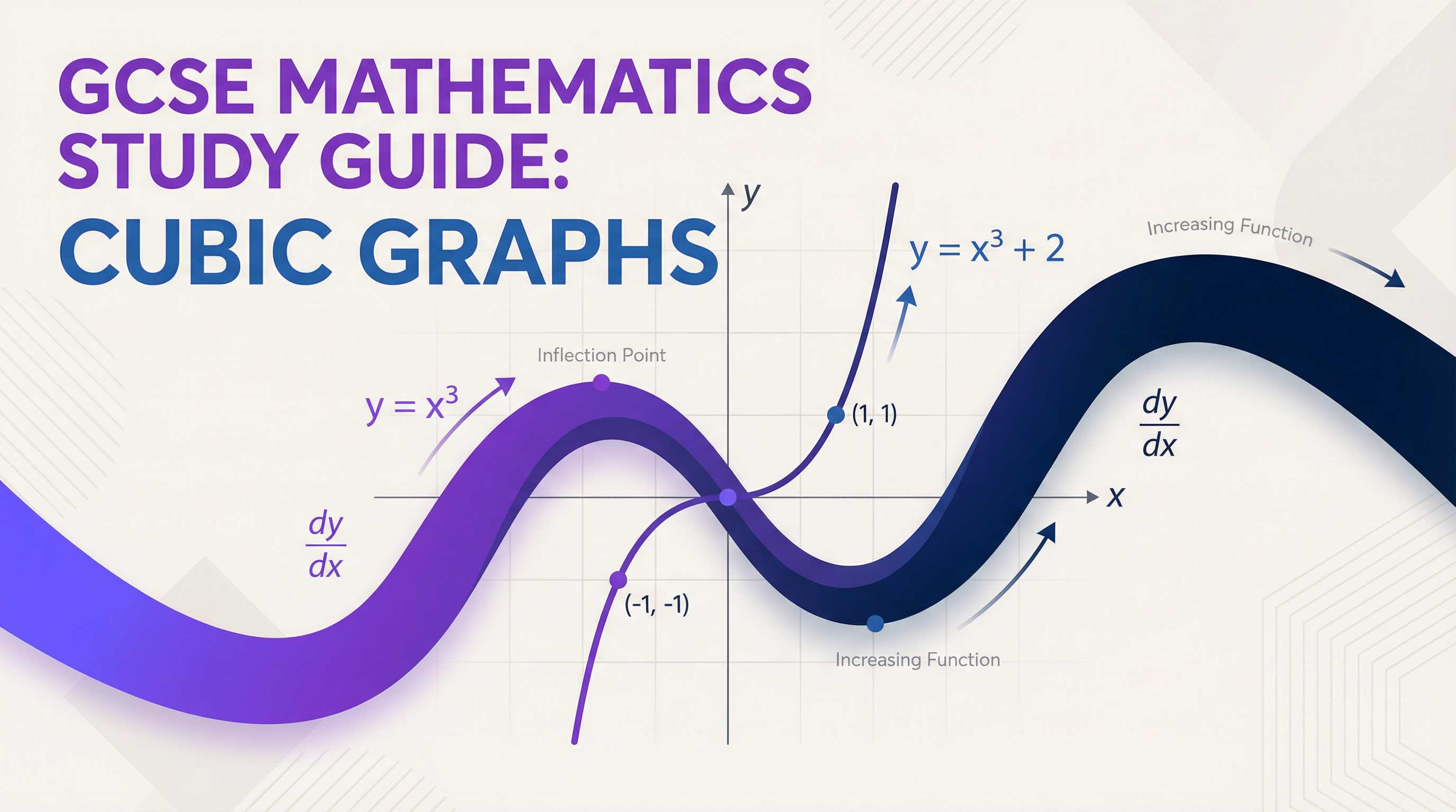
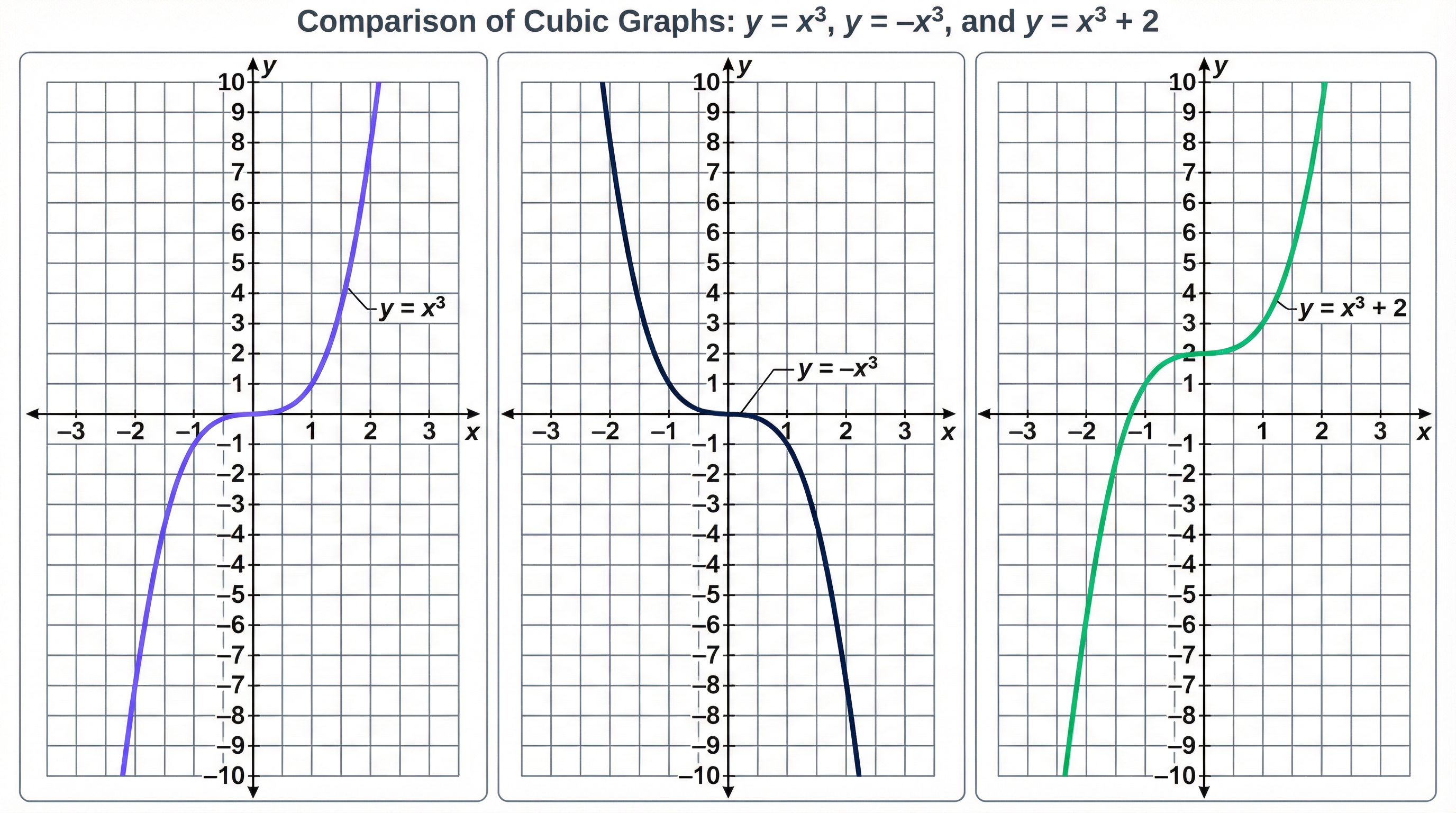
The most fundamental aspect of a cubic graph is its characteristic 'S' shape. This shape arises from the nature of the cubic function. For a positive cubic function, where the x³ term is positive (e.g., y = x³), the graph starts in the bottom-left quadrant, passes through a point of inflection, and continues to the top-right quadrant. Conversely, for a negative cubic function (e.g., y = -x³), the graph is reflected in the x-axis, starting in the top-left and finishing in the bottom-right.
Example: The graph of y = x³ passes through the origin (0,0). When x is negative, x³ is also negative. When x is positive, x³ is positive. This creates the classic S-shape.
Concept 2: Plotting from a Table of Values
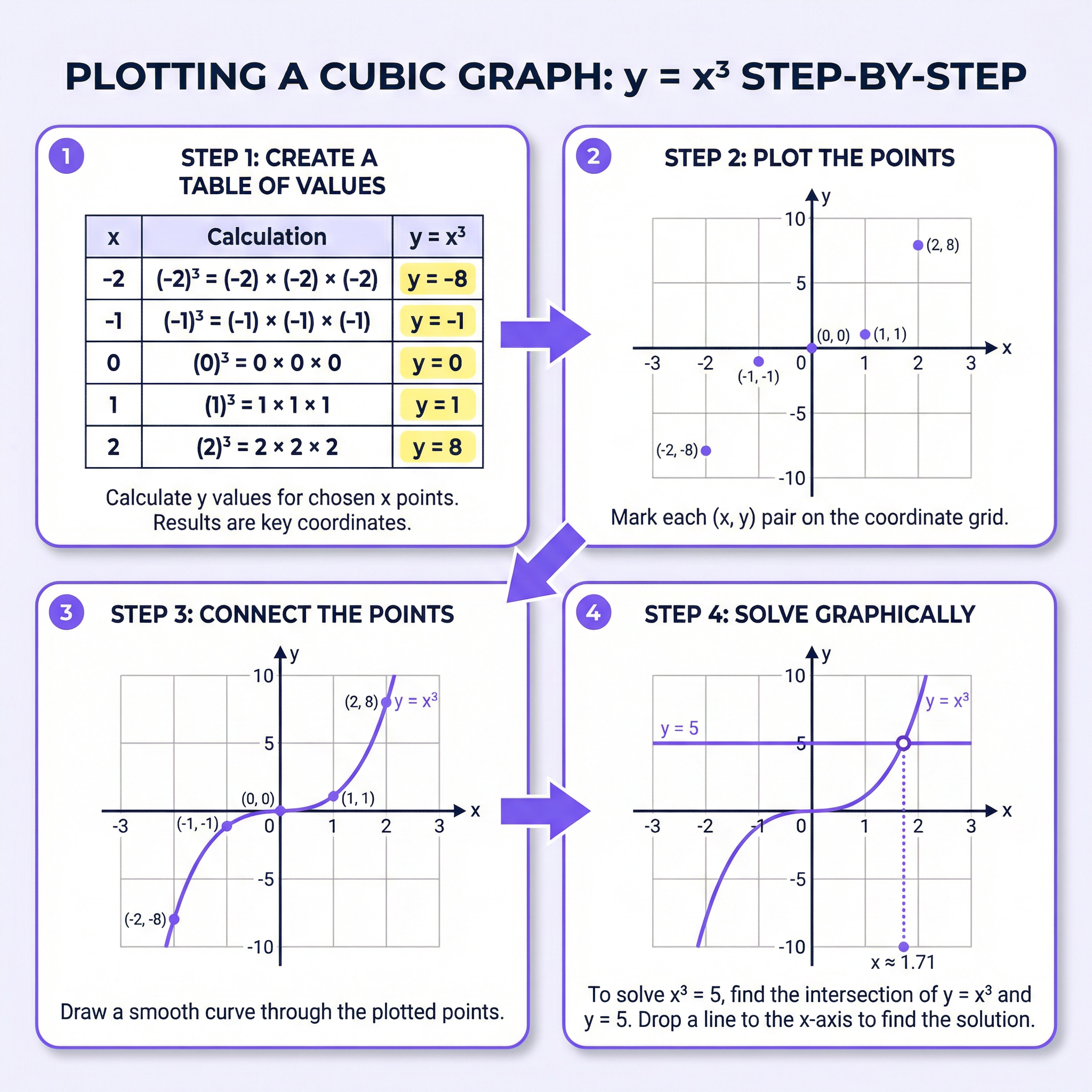
Examiners frequently test your ability to plot a cubic graph from a given table of values. This process has three distinct stages, each typically worth one mark.
- Calculating y-values: You must substitute the given x-values into the cubic equation to find the corresponding y-values. Be extremely careful with negative numbers. For example, if y = x³ and x = -2, then y = (-2)³ = -8. A common error is to calculate this as 8.
- Plotting Points: Each (x, y) pair must be plotted accurately on the coordinate grid. Examiners allow a tolerance of ±½ a small square. Use a sharp pencil and mark each point with a neat cross or dot.
- Drawing the Curve: This is a crucial step. You must connect the points with a single, smooth, continuous curve. Do not use a ruler to join the points, and avoid any 'feathery' or double lines. The curve should flow naturally through the plotted points.
Concept 3: Solving Equations Graphically
Once you have drawn your cubic graph, you can use it to solve equations. For example, to solve the equation x³ - 2x = 3, you would draw the line y = 3 on the same axes as your graph of y = x³ - 2x. The x-coordinates of the points where the line and the curve intersect are the solutions to the equation. You must show your method clearly by drawing the horizontal line and then drawing vertical lines from the intersection points down to the x-axis.
Mathematical/Scientific Relationships
- General Form: The general form of a cubic function is y = ax³ + bx² + cx + d, where a, b, c, and d are constants and a ≠ 0.
- Roots: The roots of a cubic function are the x-values where the graph crosses the x-axis (i.e., where y = 0). A cubic function can have one, two, or three real roots.
- Y-intercept: The y-intercept is the point where the graph crosses the y-axis. This occurs when x = 0, so the y-intercept is always at the point (0, d).
Practical Applications
While cubic functions might seem abstract, they are used to model various real-world phenomena. In physics, they can describe the relationship between the length of a pendulum and its period. In economics, they can model cost functions, where the cost of production changes at different rates. In engineering, the bending of beams can sometimes be described by cubic equations. Understanding their shape and properties provides a powerful tool for modelling complex systems.